color1 = ['#7fc97f', '#beaed4', '#fdc086', '#ffff99',
'#386cb0', '#f0027f', '#bf5b17', '#666666']
color2 = ['#1b9e77', '#d95f02', '#7570b3', '#e7298a',
'#66a61e', '#e6ab02', '#a6761d', '#666666']
color3 = ['#a6cee3', '#1f78b4', '#b2df8a', '#33a02c',
'#fb9a99', '#e31a1c', '#fdbf6f', '#ff7f00']
color4 = ['#fbb4ae', '#b3cde3', '#ccebc5', '#decbe4',
'#fed9a6', '#ffffcc', '#e5d8bd', '#fddaec']
color5 = ['#66c2a5', '#fc8d62', '#8da0cb', '#e78ac3',
'#a6d854', '#ffd92f', '#e5c494', '#b3b3b3']
color6 = ['#b3e2cd', '#fdcdac', '#cbd5e8', '#f4cae4',
'#e6f5c9', '#fff2ae', '#f1e2cc', '#cccccc']
color7 = ['#e41a1c', '#377eb8', '#4daf4a', '#984ea3',
'#ff7f00', '#ffff33', '#a65628', '#f781bf']
color8 = ['#8dd3c7', '#ffffb3', '#bebada', '#fb8072',
'#80b1d3', '#fdb462', '#b3de69', '#fccde5']
color2l = ['red', 'green', '#78a6cd', '#ccebc5', '#decbe4']
color_seq1 = ['#f7fcfd', '#e5f5f9', '#ccece6', '#99d8c9',
'#66c2a4', '#41ae76', '#238b45', '#005824']
color_seq2 = ['#fff7ec', '#fee8c8', '#fdd49e', '#fdbb84',
'#fc8d59', '#ef6548', '#d7301f', '#990000']
color_seq3 = ['#f7fbff', '#deebf7', '#c6dbef', '#9ecae1',
'#6baed6', '#4292c6', '#2171b5', '#084594']
color_seq4 = ['#f7fcf5', '#e5f5e0', '#c7e9c0', '#a1d99b',
'#74c476', '#41ab5d', '#238b45', '#005a32']
color_seq5 = ['#fff5f0', '#fee0d2', '#fcbba1', '#fc9272',
'#fb6a4a', '#ef3b2c', '#cb181d', '#99000d']
color_seq6 = ['#fff5eb', '#fee6ce', '#fdd0a2', '#fdae6b',
'#fd8d3c', '#f16913', '#d94801', '#8c2d04']
color_seq7 = ['#ffffd9', '#edf8b1', '#c7e9b4', '#7fcdbb',
'#41b6c4', '#1d91c0', '#225ea8', '#0c2c84']
color_seq8 = ['#fff7fb', '#ece2f0', '#d0d1e6', '#a6bddb',
'#67a9cf', '#3690c0', '#02818a', '#016450']
color_seq9 = ['#ffffff', '#f0f0f0', '#d9d9d9', '#bdbdbd',
'#969696', '#737373', '#525252', '#252525']
color_div1 = ['#8c510a', '#bf812d', '#dfc27d', '#f6e8c3',
'#c7eae5', '#80cdc1', '#35978f', '#01665e']
color_div2 = ['#c51b7d', '#de77ae', '#f1b6da', '#fde0ef',
'#e6f5d0', '#b8e186', '#7fbc41', '#4d9221']
color_div3 = ['#762a83', '#9970ab', '#c2a5cf', '#e7d4e8',
'#d9f0d3', '#a6dba0', '#5aae61', '#1b7837']
color_div4 = ['#b2182b', '#d6604d', '#f4a582', '#fddbc7',
'#d1e5f0', '#92c5de', '#4393c3', '#2166ac']
color_div5 = ['#b2182b', '#d6604d', '#f4a582', '#fddbc7',
'#e0e0e0', '#bababa', '#878787', '#4d4d4d']
color_div6 = ['#d73027', '#f46d43', '#fdae61', '#fee090',
'#e0f3f8', '#abd9e9', '#74add1', '#4575b4']
color_div7 = ['#d73027', '#f46d43', '#fdae61', '#fee08b',
'#d9ef8b', '#a6d96a', '#66bd63', '#1a9850']
color_div8 = ['#d53e4f', '#f46d43', '#fdae61', '#fee08b',
'#e6f598', '#abdda4', '#66c2a5', '#3288bd']
def draw_bar_single(var_x, var_y, label_x, label_y, titre, col_titre='MidnightBlue', pos_titre='center', titre_y=1, titre_x=0.5, title_linespacing=1.0, legend_out=False, col_bar='teal', alpha_bar=0.7, base_mtick=1.0, xdate_available=False, alpha_grid=0.3):
"""
Mettre xdate_available=True pour orienté le texte des graduations sur l'axe x
"""
x = var_x
y = var_y
_ = plt.title(titre, color=col_titre, loc=pos_titre, y=titre_y, x=titre_x,
linespacing=title_linespacing, fontdict={'size': 20, 'weight': 500})
loc = mtick.MultipleLocator(base=base_mtick)
ax.xaxis.set_major_locator(loc)
if xdate_available:
fig.autofmt_xdate(bottom=0.2, rotation=30, ha='right', which='major')
_ = plt.xlabel(label_x, labelpad=15, color='gray', fontdict={'size': 16})
_ = plt.ylabel(label_y, labelpad=15, color='gray', fontdict={'size': 16})
if legend_out:
_ = plt.legend(bbox_to_anchor=(1.03, 1.0), loc='upper left')
_ = plt.bar(x, y, align='center', color=col_bar, alpha=alpha_bar)
_ = plt.grid(linestyle='--', alpha=alpha_grid)
###########################
def draw_plot(var_y, var_x, label_x, label_y, titre, nb=1, col_titre='MidnightBlue', pos_titre='center', titre_y=1, titre_x=0.5, title_linespacing=1.0, legend_out=False, col_bar='teal', alpha_bar=0.7, base_mtick=1.0, xdate_available=False, alpha_grid=0.3):
"""
Mettre xdate_available=True pour orienté le texte des graduations sur l'axe x
"""
y = var_y
x = var_x
_ = plt.title(titre, color=col_titre, loc=pos_titre, y=titre_y, x=titre_x,
linespacing=title_linespacing, fontdict={'size': 20, 'weight': 500})
loc = mtick.MultipleLocator(base=base_mtick)
ax.xaxis.set_major_locator(loc)
if xdate_available:
fig.autofmt_xdate(bottom=0.2, rotation=30, ha='right', which='major')
_ = plt.xlabel(label_x, labelpad=15, color='gray', fontdict={'size': 16})
_ = plt.ylabel(label_y, labelpad=15, color='gray', fontdict={'size': 16})
if legend_out:
ax.legend(bbox_to_anchor=(1.03, 1.0), loc='upper left')
ax.plot(y, x, color=col_bar, alpha=alpha_bar)
ax.grid(linestyle='--', alpha=alpha_grid)
################################
def draw_bar_several(dfgroupby, label_x, label_y, titre, col_titre='MidnightBlue', pos_titre='center', titre_y=1.02, titre_x=0.5, title_linespacing=1, legend_out=False, legend_pers=False, legend=None, xticks_rotation='horizontal', base_mtick=1.0, g_stacked=False, g_stacked_perc=False, g_width=0.8, g_kind='bar', g_color=color1, alpha_grid=0.3):
if g_stacked_perc:
plt.plot = dfgroupby.groupby(level=0).apply(lambda x: 100 * x / x.sum()).unstack().plot(
kind=g_kind,
stacked=g_stacked,
width=g_width,
color=g_color
)
plt.gca().yaxis.set_major_formatter(mtick.PercentFormatter())
else:
plt.plot = dfgroupby.unstack().plot(
kind=g_kind,
stacked=g_stacked,
width=g_width,
color=g_color
)
if legend_out:
_ = plt.legend(bbox_to_anchor=(1.03, 1.0), loc='upper left')
if legend_pers:
_ = plt.legend(legend, bbox_to_anchor=(1.03, 1.0), loc='upper left')
_ = plt.title(titre, color=col_titre, loc=pos_titre, y=titre_y, x=titre_x,
linespacing=title_linespacing, fontdict={'size': 20, 'weight': 500})
_ = plt.xticks(rotation=xticks_rotation)
loc = mtick.MultipleLocator(base=base_mtick)
ax.xaxis.set_major_locator(loc)
_ = plt.xlabel(label_x, labelpad=15, color='gray', fontdict={'size': 16})
_ = plt.ylabel(label_y, labelpad=15, color='gray', fontdict={'size': 16})
_ = plt.grid(linestyle='--', alpha=alpha_grid)
def draw_bar_pie(titre, labels_in, size_in, explode_in, titre_legend, z, a=1, b=1, c=1, color_titre='MidnightBlue', def_angle=90, titre_x=0.5, titre_y=1.05, title_linespacing=1, legend_available=True, pos_titre='center', size_titre=18, color_perc='white', size_perc=16, loc_legend="center left", bbox_legend=(1, 0, 0.5, 1), g_color=color5):
"""
fig=plt.figure(figsize=(18,6))
"""
labels = labels_in
size = size_in
explode = explode_in
z = fig.add_subplot(a, b, c)
patches, texts, autotexts = z.pie(
size, explode=explode, autopct='%1.1f%%', shadow=True, startangle=def_angle, colors=g_color)
if legend_available:
legend = z.legend(patches, labels,
title=titre_legend,
loc=loc_legend,
bbox_to_anchor=bbox_legend)
# Equal aspect ratio ensures that pie is drawn as a circle.
z.axis('equal')
_ = plt.setp(autotexts, color=color_perc, size=size_perc, weight="bold")
z.set_title(titre, color=color_titre, loc='center', y=titre_y, x=titre_x,
linespacing=title_linespacing, fontdict={'size': size_titre, 'weight': 500})
def draw_scatter(df, col_df_x, col_df_y, label_x, label_y, titre, col_titre='MidnightBlue', pos_titre='center', titre_y=1.02, titre_x=0.5, title_linespacing=1, legend_out=False, xticks_rotation='horizontal', base_mtick=1.0, g_stacked=False, g_stacked_perc=False, color_scatter='teal', alpha_grid=0.3):
params = {
'figure.figsize': (16, 6),
}
pylab.rcParams.update(params)
df.plot(
kind='scatter',
x=col_df_x,
y=col_df_y,
color=color_scatter
)
if legend_out:
plt.legend(bbox_to_anchor=(1.03, 1.0), loc='upper left')
_ = plt.title(titre, color=col_titre, loc=pos_titre, y=titre_y, x=titre_x,
linespacing=title_linespacing, fontdict={'size': 20, 'weight': 500})
_ = plt.xticks(rotation=xticks_rotation)
loc = mtick.MultipleLocator(base=base_mtick)
ax.xaxis.set_major_locator(loc)
_ = plt.xlabel(label_x, labelpad=15, color='gray', fontdict={'size': 16})
_ = plt.ylabel(label_y, labelpad=15, color='gray', fontdict={'size': 16})
_ = plt.grid(linestyle='--', alpha=alpha_grid)
# _=plt.show()
def draw_options(titre, label_x, label_y, col_titre='MidnightBlue', pos_titre='center', titre_y=1.02, titre_x=0.5, title_linespacing=1, legend_out=False, legend_pers=False, legend=None, alpha_grid=0.3):
_ = plt.title(titre, color=col_titre, loc=pos_titre, y=titre_y, x=titre_x,
linespacing=title_linespacing, fontdict={'size': 20, 'weight': 500})
_ = plt.xlabel(label_x, labelpad=15, color='gray', fontdict={'size': 16})
_ = plt.ylabel(label_y, labelpad=15, color='gray', fontdict={'size': 16})
if legend_out:
_ = plt.legend(bbox_to_anchor=(1.03, 1.0), loc='upper left')
if legend_pers:
_ = plt.legend(legend_p, bbox_to_anchor=(1.03, 1.0), loc='upper left')
_ = plt.grid(linestyle='--', alpha=alpha_grid)
# this plots multiple seaborn histograms on different subplots
def plot_multiple_histograms(df, cols):
num_plots = len(cols)
num_cols = math.ceil(np.sqrt(num_plots))
num_rows = math.ceil(num_plots/num_cols)
fig, axs = plt.subplots(num_rows, num_cols)
for ind, col in enumerate(cols):
i = math.floor(ind/num_cols)
j = ind - i*num_cols
if num_rows == 1:
if num_cols == 1:
sns.distplot(df[col], kde=True, ax=axs)
else:
sns.distplot(df[col], kde=True, ax=axs[j])
else:
sns.distplot(df[col], kde=True, ax=axs[i, j])
def gini(arr):
count = arr.size
coefficient = 2 / count
indexes = np.arange(1, count + 1)
weighted_sum = (indexes * arr).sum()
total = arr.sum()
constant = (count + 1) / count
return coefficient * weighted_sum / total - constant
def lorenz_f(arrg, title, xlabel, ylabel, arrg2=None, arrg3=None, arrg4=None, nb=1, fs=8, title_lorenz=None):
patterns = ('X', '\\', '-', '+', 'O', '*', '.')
fig = plt.figure(figsize=(fs, fs))
x1 = [0, 1]
y1 = [0, 1]
ax = fig.add_subplot(111)
_ = ax.plot(x1, y1, color='black', alpha=0.7)
_ = ax.set(xlim=(0, 1), ylim=(0, 1))
# _=ax.axis('equal')
_ = ax.tick_params(axis='both', which='major', labelsize=14)
plt.gca().xaxis.set_major_formatter(mtick.PercentFormatter(1.0))
plt.gca().yaxis.set_major_formatter(mtick.PercentFormatter(1.0))
_ = plt.ylabel(ylabel, color='gray', labelpad=10, fontdict={'size': 16})
_ = plt.xlabel(xlabel, color='gray', labelpad=15, fontdict={'size': 16})
_ = plt.title(title, y=1.02, fontdict={'size': 20, 'weight': 500})
if nb == 2:
arrge = [arrg, arrg2]
if nb == 3:
arrge = [arrg, arrg2, arrg3]
if nb == 4:
arrge = [arrg, arrg2, arrg3, arrg4]
for i in range(nb):
if nb == 1:
arr = arrg
else:
arr = arrge[i]
arr = arr.sort_values()
n = len(arr)
lorenz = np.cumsum(arr) / arr.sum()
lorenz = np.append([0], lorenz)
xaxis = np.linspace(0, 1, n+1)
if title_lorenz:
_ = ax.plot(xaxis, lorenz, drawstyle='steps-post',
color=color2l[i], label='Courbe de Lorenz '+title_lorenz[i])
else:
_ = ax.plot(xaxis, lorenz, drawstyle='steps-post',
color=color2l[i], label='Courbe de Lorenz')
if nb == 1:
_ = ax.fill_between(xaxis, xaxis, lorenz, alpha=0.6, hatch="X",
color='teal', label='Surface de concentration')
_ = ax.fill_between(np.linspace(0, 1, len(lorenz)),
lorenz, color='gray', alpha=0.3)
else:
_ = ax.fill_between(xaxis, xaxis, lorenz,
hatch=patterns[i], color=color2l[i], alpha=0.3)
gini_value = gini(arr)
if title_lorenz:
r = 0.7-(i/20)
_ = ax.text(0.1, r, "Gini "+str(title_lorenz[i]) + " = "+str(
round(gini_value, 2)), fontsize=16, color=color2l[i], weight='semibold')
else:
_ = ax.text(0.2, 0.6, "Gini = " + str(round(gini_value, 2)),
fontsize=18, color='darkred', weight='semibold')
patch = []
if nb == 1:
a_patch = mpatches.Patch(
color='teal', alpha=0.6, hatch="X", label='Surface de concentration')
b_patch = mpatches.Patch(
color=color2l[0], label='Courbe de Lorenz')
_ = plt.legend(handles=[a_patch, b_patch])
else:
if title_lorenz:
p = mpatches.Patch(
color=color2l[i], label='Courbe de Lorenz '+title_lorenz[i])
patch.append(p)
_ = plt.legend(handles=patch)
else:
p = mpatches.Patch(color=color2l[i], label='Courbe de Lorenz')
patch.append(p)
_ = plt.legend(handles=patch)
_ = ax.legend(loc='upper left', bbox_to_anchor=(0.02, 0.98), fontsize=12,
frameon=True, ncol=1, fancybox=True, framealpha=1, shadow=True, borderpad=0.5)
_ = ax.grid(linestyle='--', alpha=0.4)
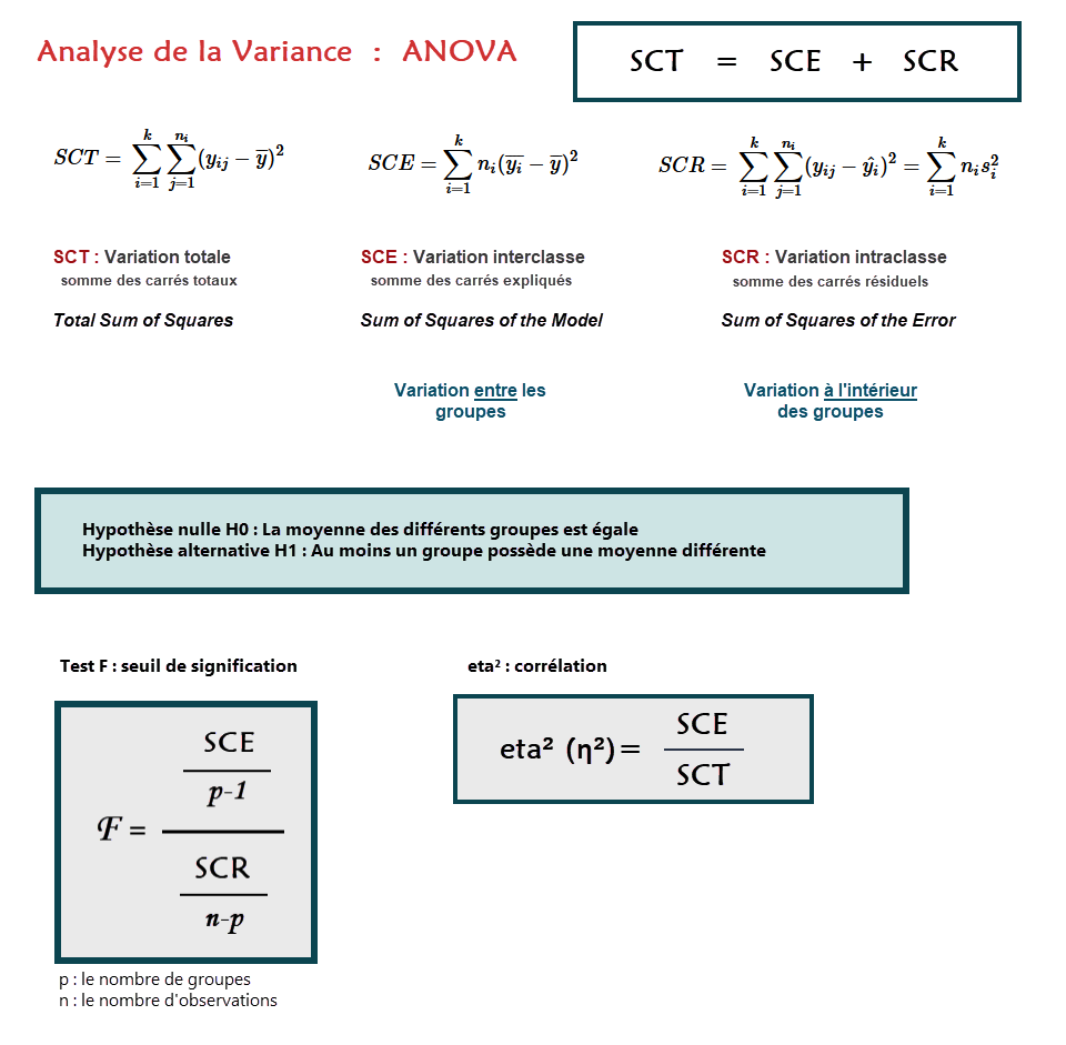
def eta_squared(x, y):
moyenne_y = y.mean()
classes = []
for classe in x.unique():
yi_classe = y[x == classe]
classes.append({'ni': len(yi_classe),
'moyenne_classe': yi_classe.mean()})
SCT = sum([(yj-moyenne_y)**2 for yj in y])
SCE = sum([c['ni']*(c['moyenne_classe']-moyenne_y)**2 for c in classes])
return SCE/SCT
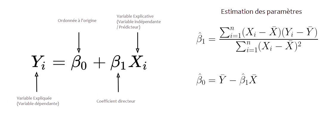
def linear_regression(x, y):
N = len(x)
x_mean = x.mean()
y_mean = y.mean()
B1_num = ((x - x_mean) * (y - y_mean)).sum()
B1_den = ((x - x_mean)**2).sum()
B1 = B1_num / B1_den
B0 = y_mean - (B1*x_mean)
sign = '+'
if B1 < 0:
sign = '-'
B3 = -B1
else:
B3 = B1
reg_line = 'y = {} {} {}β'.format(B0, sign, round(B3, 3))
return (B0, B1, reg_line)
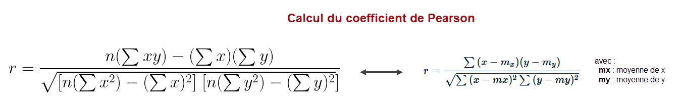
def corr_coef(x, y):
N = len(x)
num = (N * (x*y).sum()) - (x.sum() * y.sum())
den = np.sqrt((N * (x**2).sum() - x.sum()**2) * (N * (y**2).sum() - y.sum()**2))
R = num / den
return R
def linear_reg_aff(x,y):
B0, B1, reg_line = linear_regression(x, y)
R = corr_coef(x, y)
text="Droite de régression : "+str(reg_line)+"\nCoef. de corrélation R : "+str(R)+"\nCoef. de détermination R² : "+str(R**2)
return print(text)
def graph_droite_regression(dataset, x, y, text_x, text_y, titre, axes_x, axes_y,
size_col, sizes_taille, titre_leg="",
leg_x=0.1, leg_y=0.1, loc_leg='lower left', axe="ax1",
inter=np.arange(100), inter_droite=np.arange(100), size_title=20,
xlim_p=None, ylim_p=None, droite_reg=True):
x1=dataset[x]
y1=dataset[y]
B0, B1, reg_line = linear_regression(x1,y1)
R = corr_coef(x1,y1)
sign = '+'
if B1 < 0:
sign = '-'
B3 = -B1
else:
B3 = B1
dic_ax = { "ax1":ax1, "ax2":ax2 }
X=dic_ax[axe]
X = plt.gca()
text = "Moyenne X : {}\nMoyenne Y : {}\nR : {}\nR^2 : {}\ny = {} {} {}X".format(
round(x1.mean(), 2),
round(y1.mean(), 2),
round(R, 4),
round(R**2, 4),
round(B0, 3),
sign,
round(B3, 3))
if droite_reg:
_ = plt.text(x=text_x, y=text_y, s=text, fontsize=12, bbox={'facecolor': 'grey', 'edgecolor':'black', 'boxstyle':'round,pad=1', 'alpha': 0.2, 'pad': 10})
_ = X.plot(inter_droite, [B0 + B1*x for x in inter_droite], c = 'r', linewidth=5, alpha=.5, solid_capstyle='round')
_ = sns.scatterplot(data=dataset, x=x, y=y, marker="o", size=size_col, sizes=sizes_taille, ax=X)
if xlim_p:
_ = plt.xlim(xlim_p)
if ylim_p:
_ = plt.ylim(ylim_p)
_ = plt.xticks(inter)
_ = plt.xlabel(axes_x, color='gray', labelpad=15, fontdict={'size': 16})
_ = plt.ylabel(axes_y, color='gray', labelpad=15, fontdict={'size': 16})
_ = plt.title(titre, y=1.02, fontdict={'size': size_title, 'weight': 500})
_ = plt.legend(title=titre_leg, loc=loc_leg, bbox_to_anchor=(leg_x, leg_y),frameon=True, ncol=1, fancybox=True, framealpha=1, shadow=True, borderpad=1,fontsize=12)